
Zero‑Shot LQR

Zero-Shot Linear Quadratic Regulation from Reward-Free Data: Structured Successor Features with Stability and Finite-Sample Guarantees

Collect one reward-free dataset. Solve every linear-quadratic task afterwards in closed form, with no replanning, no second pass over the data, and no neural approximation.

Huy Dao1, Khanh Thai1,2, Bao Le1

1VinMotion, Vietnam
2School of Electrical and Electronic Engineering, Hanoi University of Science and Technology, Hanoi, Vietnam

VinMotionHanoi University of Science and Technology (HUST)
Paper · coming soon Code · coming soon
Exactfor noise-free persistently-exciting data
0 iterszero-iteration SF-GPI at test time
0.4 mstest-time cost, independent of $N$
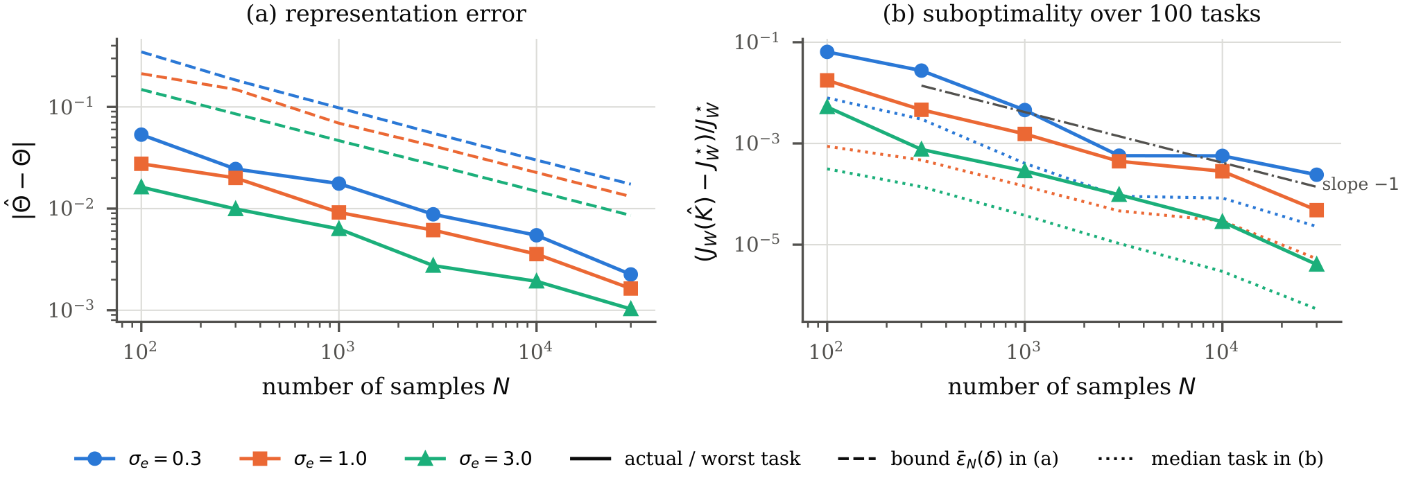
$O(\sigma_w\sqrt{\log(1/\delta)/(N\lambda_{\mathrm{PE}})})$uniform finite-sample suboptimality

Reward-Free Data Once, Any LQR Task Instantly

Classical RL and adaptive dynamic programming for the linear quadratic regulator solve one performance index at a time. Each change to the weights $(Q,R)$ forces another pass over the data and another policy iteration. We bring zero-shot reinforcement learning to LQR. A fixed-size statistic of reward-free data then solves every task exactly, without touching the data again.

Full abstract

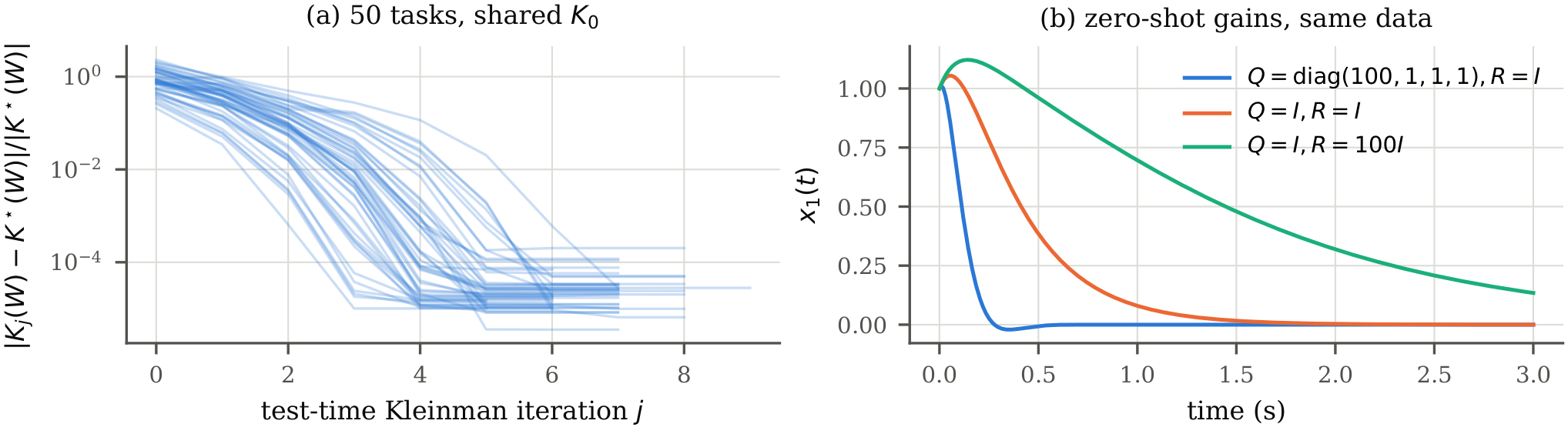
Reinforcement learning (RL) and adaptive dynamic programming (ADP) algorithms for the linear quadratic regulator (LQR) learn the optimal gain for one performance index. Each time the designer changes the weights $(Q,R)$, these algorithms must re-collect or re-process data and re-run policy iteration. Zero-shot RL instead learns a representation from reward-free interaction and reads out the optimal policy for any reward revealed at test time, without further learning. Existing zero-shot methods, however, rely on neural approximation and give no stability or optimality guarantee. This paper brings zero-shot RL to linear optimal control. For linear systems with quadratic costs, we show three facts. First, the successor features of every linear policy are exact quadratic forms. Second, the map from $(Q,R)$ to the Q-function kernel is linear, with a closed-form successor operator. Third, a fixed-size second-moment statistic of reward-free data is a sufficient zero-shot representation. On this basis, we propose a zero-shot LQR algorithm for discrete-time systems. An offline phase compresses arbitrary reward-free trajectories into the representation. A test phase maps any task $(Q,R)$, given explicitly or through reward labels, to a gain. The test phase uses either a data-free policy iteration or, with no iteration, successor-feature generalized policy improvement (GPI). We prove three guarantees. With noise-free persistently exciting data, the returned gains equal the Riccati-optimal gains for all tasks simultaneously. The GPI policy is exponentially stabilizing and no worse than any library policy. Under sub-Gaussian process noise, the following holds with probability $1-\delta$ and uniformly over a compact task set: the gains are stabilizing, and their relative suboptimality is $O\!\big(\sigma_w\sqrt{\log(1/\delta)/(N\lambda_{\mathrm{PE}})}\big)$. Here $N$ is the number of samples and $\lambda_{\mathrm{PE}}$ is the persistency-of-excitation level. A certificate computed from data verifies stability and suboptimality for each task. The framework extends to continuous-time systems through an integral-data Gram representation and a data-free Kleinman iteration. On the unstable batch reactor, simulations confirm exactness to machine precision over 200 random tasks and the predicted sample complexity. The test-time cost per task stays at $0.4\,$ms for every data length, whereas per-task off-policy Q-learning takes $14$–$359\,$ms.

01
Exact structured successor features
The successor features of every linear policy are exact quadratic forms. The map from a task $(Q,R)$ to its Q-function kernel is a closed-form, task-linear operator $\mathcal{L}_K$. Nothing here is approximated by a network.
02
Two-phase zero-shot algorithm
An offline phase compresses reward-free trajectories into a fixed-size representation. The test phase then maps any task to a gain, either by data-free policy iteration (Mode PI) or by zero-iteration SF-GPI (Mode GPI).
03
Provable guarantees
Noise-free persistently exciting (PE) data give exactly Riccati-optimal gains for all tasks at once. SF-GPI is exponentially stabilizing. Under sub-Gaussian noise, a certificate computed from data bounds the suboptimality uniformly over tasks.
04
Validated on an unstable batch reactor
One dataset solves 200 random tasks to machine precision. The test-time cost stays at $0.4\,$ms per task, against $14$–$359\,$ms for per-task off-policy Q-learning. A continuous-time extension follows the same pattern.

Compress One Reward-Free Dataset, Then Map Any Task in Closed Form

The offline phase accumulates second moments of reward-free, off-policy trajectories and, optionally, a small library of successor operators for anchor tasks. At test time, any task is mapped to a stabilizing gain without touching the data or the plant again.
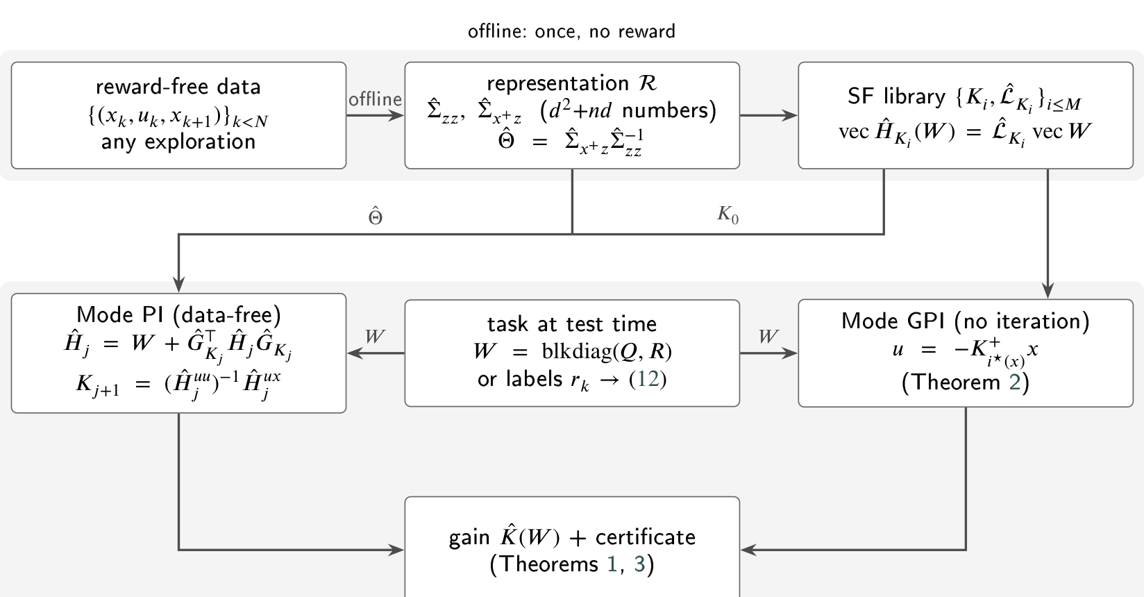
Zero-shot LQR pipeline: an offline phase compresses reward-free data into a fixed-size representation and an SF library; a test-time phase maps any task to a gain via Mode PI or Mode GPI, with no data access or interaction
Fig. 2Zero-shot LQR. The offline phase compresses reward-free data into a fixed-size representation $(\hat\Sigma_{zz},\hat\Sigma_{x^+z})$ and, optionally, an SF library. At test time any task is mapped to a gain without touching the data or the plant. Click to open full size.

Theorem: Uniform Zero-Shot Guarantee

Assume sub-Gaussian process noise. Then the following holds with probability at least $1-\delta$, uniformly over a compact task set $\mathcal{W}$: the gains returned by Mode PI are stabilizing, and their relative suboptimality is $O\!\big(\sigma_w\sqrt{\log(1/\delta)/(N\lambda_{\mathrm{PE}})}\big)$. The statement rests on a single probabilistic event, so it needs no union bound over tasks. A certificate computed from the representation alone verifies stability and suboptimality for each individual task.

One Dataset per System, Many Controllers Read Out of It

The offline phase sees the simulator once, through reward-free rollouts driven by random inputs near an equilibrium. It never touches the simulator again. Every task $(Q,R)$ posed afterwards becomes a gain computed from the fixed-size representation alone, and that gain goes straight back into the nonlinear simulator. No retuning, no new rollouts, and no gradient steps separate one task from the next.

Cart-Pole
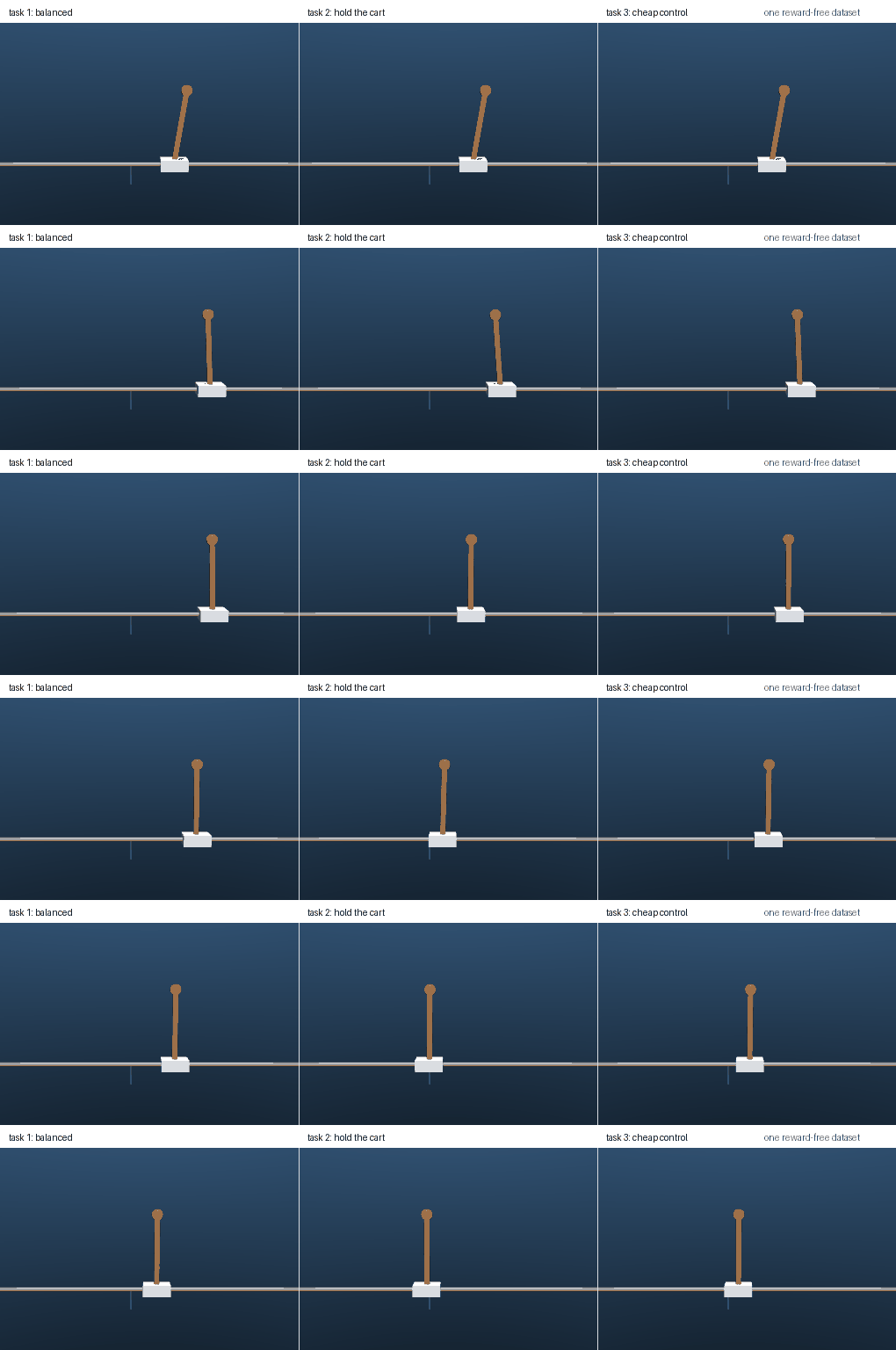
MuJoCo 3.9 cart-pole, n = 4, m = 1 50 Hz 4800 reward-free samples 0.55 ms / task
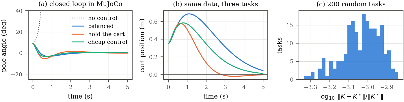
Three MuJoCo cart-pole simulations side by side, each balancing the pole with a different gain read out of the same reward-free representation
DemoOne reward-free dataset, three different performance indices. Task 2 weights cart position heavily, so it returns to the centre mark first. Task 3 buys a faster upright recovery with cheap control effort. Each gain takes about half a millisecond to compute, and uses neither the simulator nor the data.
Three panels: pole angle and cart position for the three tasks in closed loop, and a histogram of the relative gain error over 200 random tasks
Fig. 3(a) the closed loop in the nonlinear simulator, next to the uncontrolled fall. (b) the three tasks separate in how hard they pull the cart back to the centre. (c) over 200 random tasks read out of the same representation, the zero-shot gain stays within $1.4\times10^{-3}$ relative error of the Riccati gain of MuJoCo's own finite-difference linearisation, which the algorithm never sees.
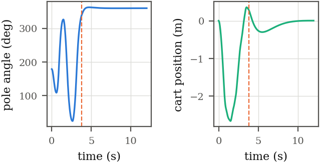
MuJoCo cart-pole starting hanging downward, pumping energy to swing up, then caught and balanced by the zero-shot LQR gain
DemoSwing-up from the hanging position. An energy-pumping law drives the pole towards upright, and once it enters the basin of the linearisation the controller hands over to the zero-shot gain of Task 1, read out of the same reward-free representation. The linear gain is only responsible for the catch; it takes over at 3.8 s and holds the pole upright afterwards.
Pole angle and cart position during swing-up, with a dashed line where the zero-shot LQR takes over
Swing-upPole angle (unwrapped) and cart position during the swing-up. The dashed line marks the hand-over to the zero-shot LQR.

Quadrotor at Hover

Hover is a harder case, and not only because the state is 12-dimensional with four inputs. The equilibrium input is nonzero, since the rotors carry the weight. The representation is therefore built on deviations from the trim point $(x^\star,u^\star)$. Regressing on raw states and inputs instead would push the missing affine term into $\hat\Theta$ and bias it.
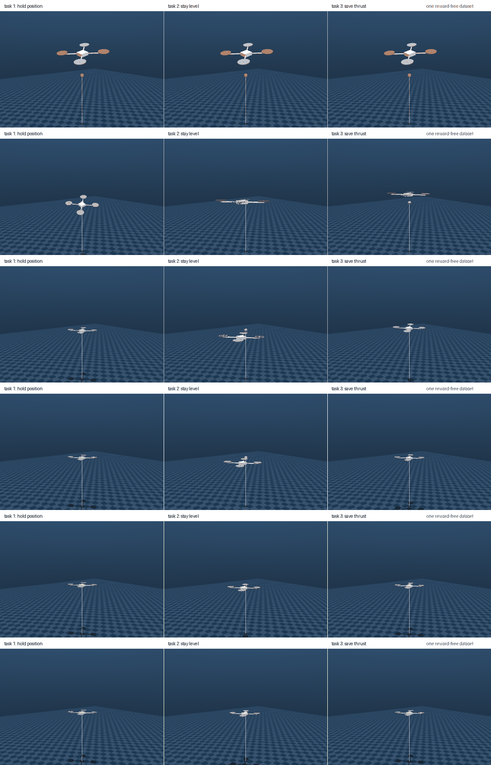
quadrotor, n = 12, m = 4 0.52 kg 100 Hz 8400 reward-free samples 0.98 ms / task
Three MuJoCo quadrotors side by side, each flying back to the same hover point with a different gain read out of the same reward-free representation
DemoThe quadrotor starts displaced and tilted, and returns to the marked hover point. Task 1 weights position, so it tilts hard to get back quickly. Task 2 weights attitude and keeps itself level, which costs it time. Task 3 penalises thrust and spends a quarter of the control effort of task 1, $0.025\,$N against $0.107\,$N of mean thrust deviation.
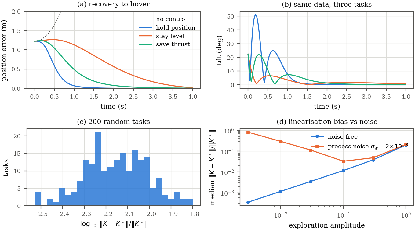
Four panels: position error and tilt for three hover tasks, a histogram of relative gain error over 200 random tasks, and gain error against exploration amplitude with and without process noise
Fig. 4(a) and (b) show the three tasks doing what their weights ask: the position-weighted gain tilts to $52^\circ$ to recover fast, while the attitude-weighted gain never exceeds $8^\circ$ and takes longer. (c) over 200 random tasks the median relative gain error is $6.8\times10^{-3}$. (d) the error against the exploration amplitude. With noise-free data the only error is the linearisation bias, which shrinks with the amplitude. Process noise pushes the other way, and the two effects meet at an interior optimum. The LTI theory covers the second effect; the first one comes from the simulator being nonlinear.

Tracking a Trajectory

Tracking needs no new theory and no new data. Around a feasible reference, the error $e=x-x_{\mathrm{ref}}$ obeys the same linear system as at hover, so the same gain closes the loop: $u=u_{\mathrm{ref}}-K\,(x-x_{\mathrm{ref}})$. The reference also comes out of the representation. For a circle, the identified model $\hat\Theta=[\hat A\;\hat B]$ gives the periodic pair $(x_{\mathrm{ref}},u_{\mathrm{ref}})$ from one square complex linear system. Nothing in the loop touches the simulator or the data after the offline phase.
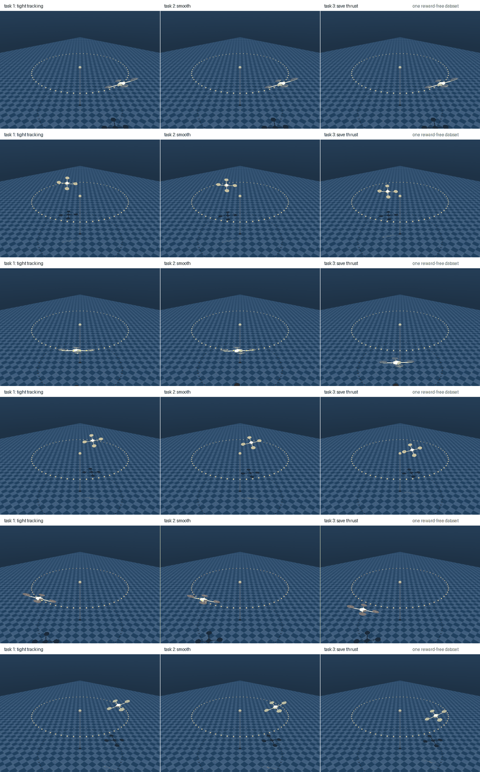
circle, r = 1 m reuses the hover dataset 3 trackers, ~1 ms each 0.12 cm RMS (tight, 6 s lap)
Three MuJoCo quadrotors flying the same circle, each with a different tracking gain read out of the same reward-free representation
DemoThe clip flies the circle at $2.1\,$m/s, a 3 s lap, where the reference tilts $26^\circ$. The three gains come from the same dataset and differ only in the weights. Their steady RMS position errors are $1.9\,$cm (tight tracking), $9.8\,$cm (smooth) and $27\,$cm (save thrust). The third tracker visibly cuts inside the ring.
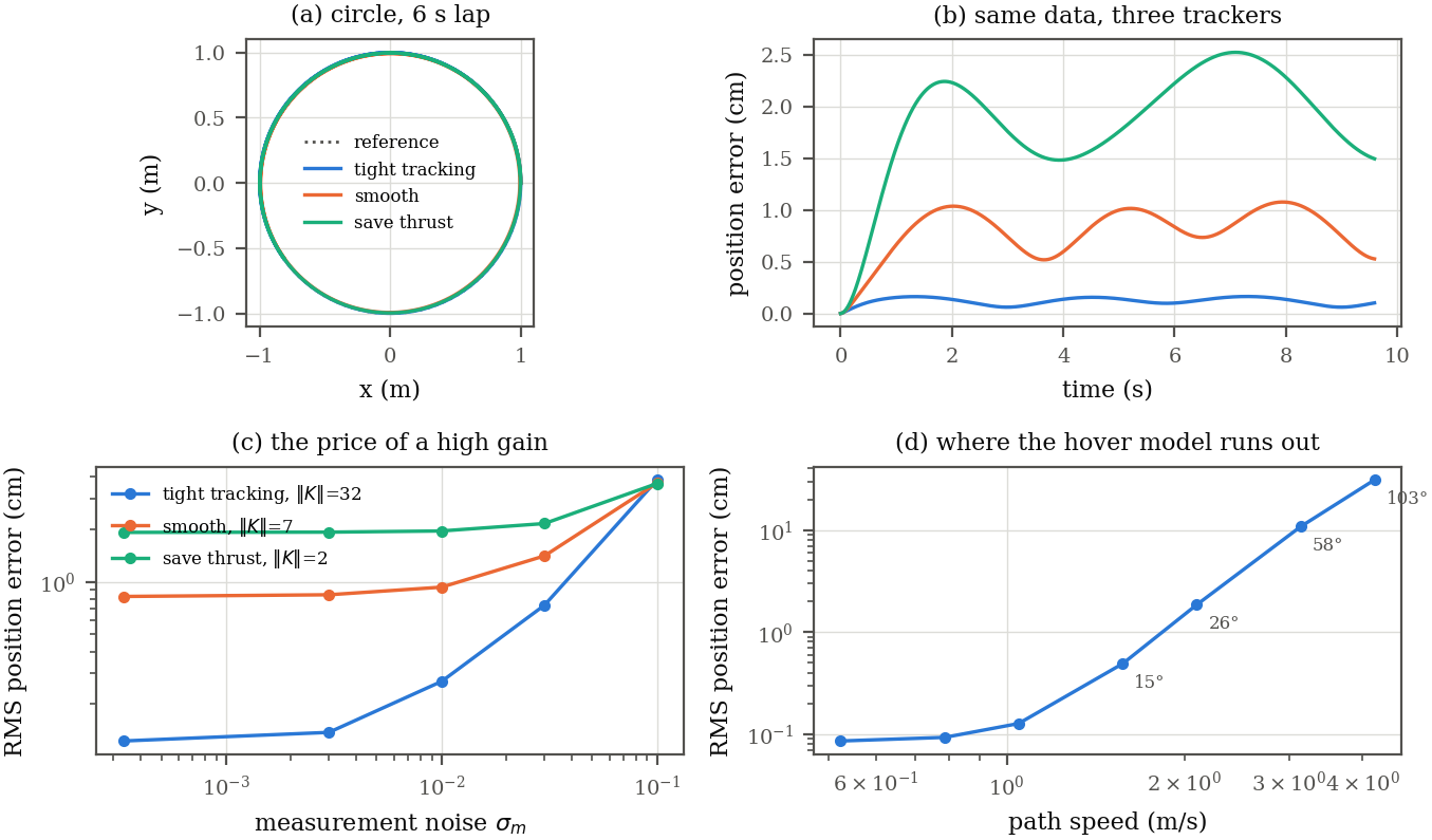
Four panels: the flown circle for three trackers, position error over time, RMS error against measurement noise for three gains, and RMS error against path speed with the reference tilt annotated
Fig. 5(a) and (b) a 6 s lap, where the three trackers reach $0.12$, $0.81$ and $1.92\,$cm RMS. (c) a high gain buys accuracy and pays for it in sensitivity to measurement noise. The tight tracker has $\|K\|=32$ against $2$ for the thrifty one, and its $16\times$ advantage in accuracy shrinks as $\sigma_m$ grows, until all three land within $6\%$ of each other at $\sigma_m=0.1$ ($3.7$ to $3.9\,$cm). (d) the tight tracker against path speed, annotated with the reference tilt. The error stays below $0.5\,$cm up to about $15^\circ$ of tilt and then grows quickly. The hover model is a local one, and this panel shows where its range ends. Past about $60^\circ$ the reference is not feasible for it at all.

Ballbot

A ballbot balances on a single ball, so it is unstable in two directions at once and every input couples a translation to a tilt: the motor pushes the ball one way and the trunk the other. The ball rolls without slipping, which ties its spin to its position. The model therefore treats it as a point of effective mass $m_b + I_b/r^2$ and loads the ball and the trunk through a tendon actuator, with the reaction torque on the trunk. The state has 8 dimensions and there are 2 inputs.
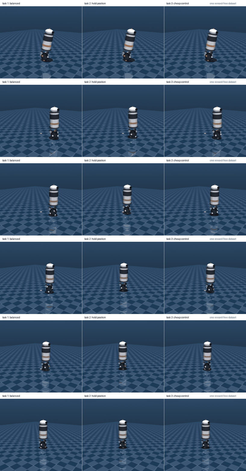
ballbot, n = 8, m = 2 50 Hz 18000 reward-free samples 1.1 ms / task
Three MuJoCo ballbots side by side, each recovering from an off-centre lean with a different gain read out of the same reward-free representation
DemoOne reward-free dataset, three performance indices. The robot starts off-centre and leaning in both directions, and each gain brings it back upright over the mark on the floor. Task 2 weights position heavily and returns closest to the origin. The ball is redrawn rolling by the distance it has travelled.
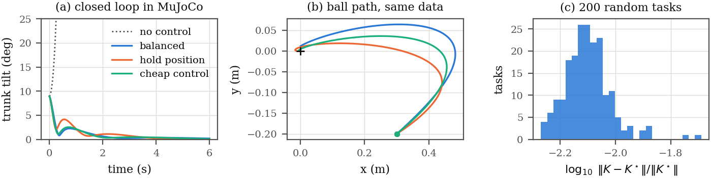
Three panels: trunk tilt for the three tasks in closed loop next to the uncontrolled fall, the path of the ball on the floor, and a histogram of the relative gain error over 200 random tasks
Fig. 6(a) the trunk tilt in the nonlinear simulator, next to the uncontrolled fall. (b) the path of the ball on the floor for the three tasks. (c) over 200 random tasks read out of the same representation the median relative gain error is $7.8\times10^{-3}$ and the worst is $2.0\times10^{-2}$, against the Riccati gain of MuJoCo's own finite-difference linearisation. The identified model is within $3.6\times10^{-3}$ of it.

Ballbot on a Circle

The ballbot also tracks a path, again with no new data and no new theory. The error around a feasible reference follows the same linear system, so the gain read out of the same representation closes the loop on the error. The reference itself, including the trunk lean that a steady turn demands, comes from the identified model: for a circle it solves one square complex system. Nothing in the loop touches the simulator or the data after the offline phase.
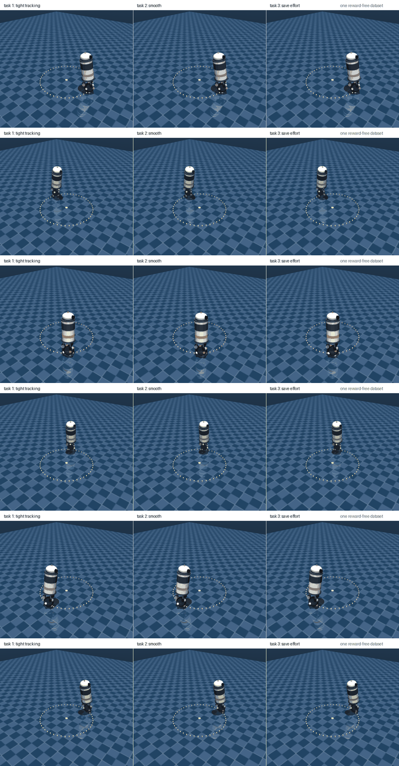
Three MuJoCo ballbots side by side, each rolling around the same dotted circle with a different tracking gain read out of the same reward-free representation
DemoThree ballbots rolling the same circle, leaning into the turn. The clip uses a 3.5 s lap so the lean and the differences between the trackers are visible. The tight tracker stays on the dotted line, and the other two drift a little off it.
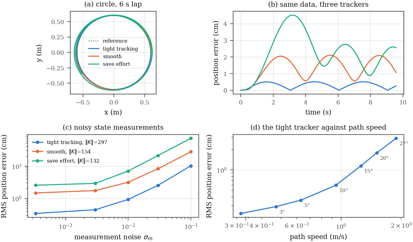
Four panels: the circle flown by three trackers, position error over time, RMS error against measurement noise for three gains, and RMS error against path speed with the reference tilt annotated
Fig. 7(a) and (b) a 6 s lap of radius 0.6 m, where the three trackers reach $0.34$, $1.48$ and $2.56\,$cm RMS. The reference leans the trunk by $4.7^\circ$. (c) the same lap with noise on the measured state. Every tracker degrades and the ordering does not change, with the tight tracker at $10\,$cm and the thriftiest at $72\,$cm when $\sigma_m=0.1$. (d) the tight tracker against path speed, annotated with the reference tilt. The error grows from $0.23\,$cm at $0.31\,$m/s to $2.9\,$cm at $1.9\,$m/s, where the reference leans $27^\circ$ and the linear model is stretched.

Humanoid on One Leg

The largest case follows MuJoCo's own LQR tutorial: the stock humanoid standing on its left leg, with the tutorial's cost, a centre-of-mass balance term plus per-joint weights. The state is 54-dimensional, with 21 torque inputs, and the foot contact is stiff, so the model is far from linear at the millimetre scale. The tutorial linearises the simulator and solves a Riccati equation. Here the offline phase only sees short reward-free episodes of random torques around the set-point, and every task is then read out of the representation. The finite-difference Riccati gain scores the result and is never used by the algorithm.

Two details matter. The keyframe is not quite a rest point, and without correcting that the data carry an affine term the linear model cannot hold. A few Newton steps on the pose and the torques remove it. The episodes also have to be short and small, four steps at about $10^{-3}$ rad, because the contact switches within a millimetre of foot height. Longer, larger episodes identify the secant of a nonlinear contact instead of the tangent that the gain needs.
humanoid, n = 54, m = 21 200 Hz 32000 reward-free samples 0.3 to 2 s / task
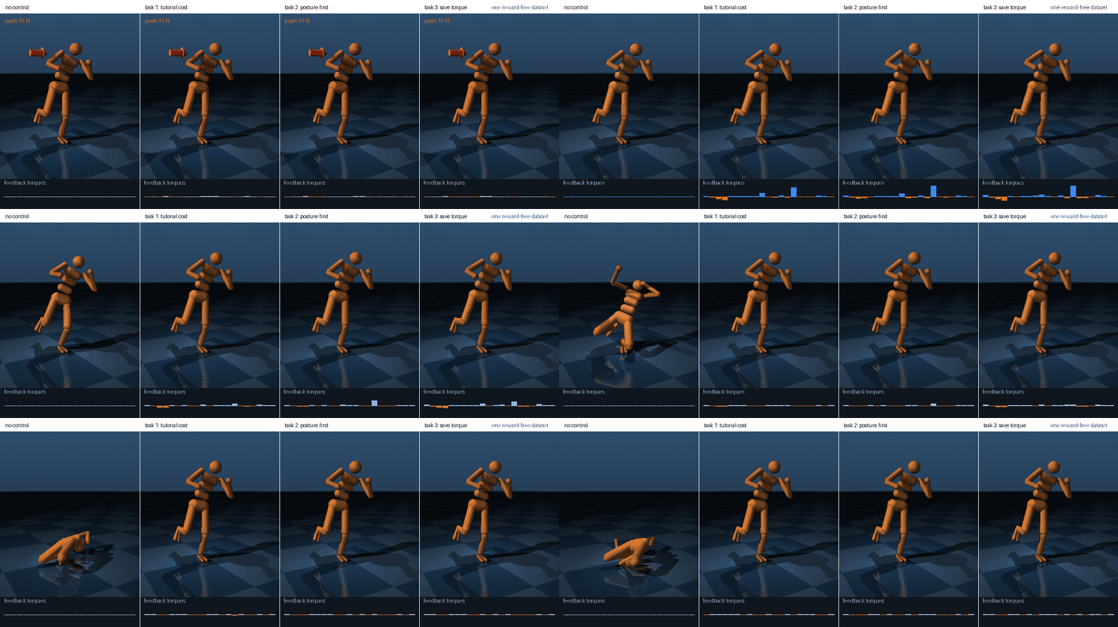
Four MuJoCo humanoids balancing on the left leg after a sideways push; the uncontrolled one falls and the three with zero-shot gains stay up
DemoA 15 N lateral push on the torso for 0.1 s, drawn as the red arrow, played at half speed. The strip under each panel shows the feedback torque of each of the 21 motors, with blue pushing one way and orange the other. Without control the humanoid falls and the strip stays flat. The three gains, read out of the same reward-free representation with different costs, answer the push with a burst of torque that is mostly at one joint, the sideways ankle of the standing leg, and hold the pose.
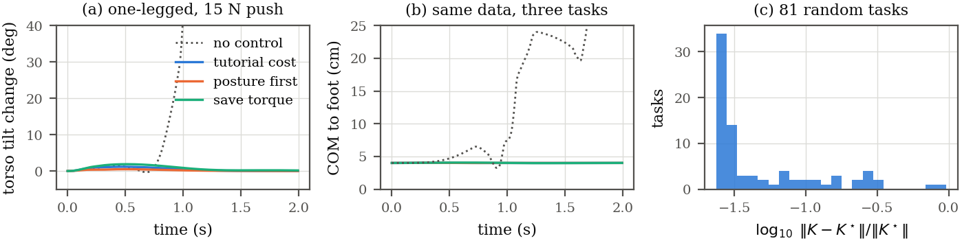
Three panels: torso tilt change after the push for the three tasks and the uncontrolled fall, distance from the centre of mass to the foot, and a histogram of the relative gain error over random tasks
Fig. 8(a) the torso tilt changes by at most $1.9^\circ$ for the three tasks, against a fall without control. (b) the centre of mass stays over the foot. (c) the relative gain error of $4.2$, $5.5$ and $11\times10^{-2}$ for the three tasks, and a median of $2.8\times10^{-2}$ over $81$ random tasks. The error is much larger than in the other demos, with a worst case near $1$, because the finite-difference model is a tangent at a stiff contact. The identified model is within $3.4\times10^{-2}$ of it. The tutorial-cost gain recovers from pushes up to $15\,$N, the same as the finite-difference Riccati gain, while the posture-first gain reaches $35\,$N and the torque-saving gain $20\,$N.

Lifting the Leg

The humanoid can also start on both feet and lift the right leg. The one-leg pose is one end of a family of equilibria: lowering the right leg toward the floor, with the rest of the body re-balanced, gives a chain of rest points that ends with the right foot touching down. Each of nine waypoints is found by Newton continuation from the previous one, and gets its own short reward-free dataset, its own representation and its own gain for the same tutorial cost. The controller follows the chain, interpolating the reference and the gain between waypoints, so the weight moves over the left leg while the foot comes up.
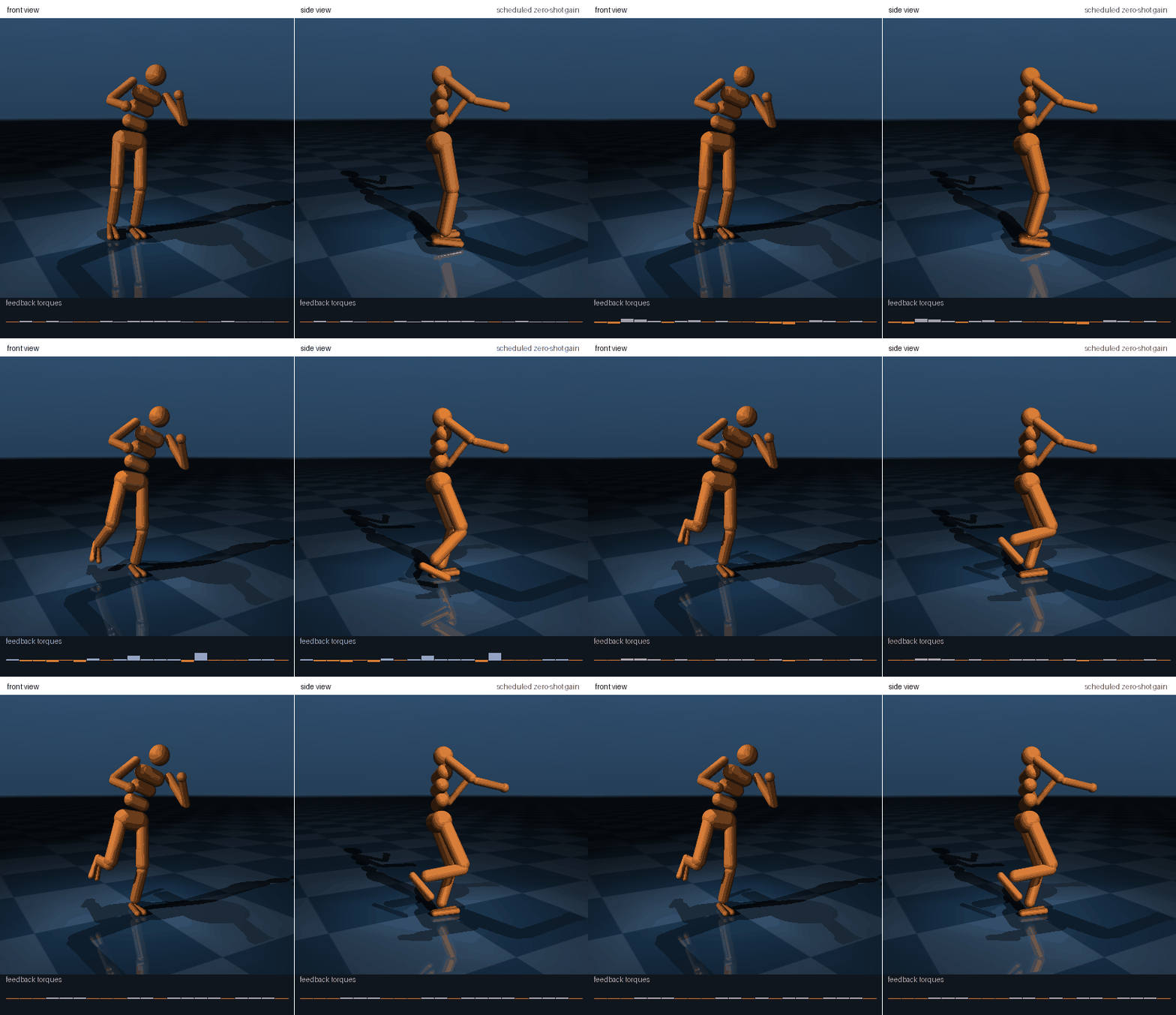
Two views of the MuJoCo humanoid starting on both feet and lifting the right leg, with a sideways push drawn as a red arrow during the lift and the feedback torques shown below
DemoThe foot rises from the floor to $0.39\,$m. A 15 N push at 2 s, during the lift, is drawn as the red arrow. The torque strip shows the motors answering it with a short burst, and the lift carries on.
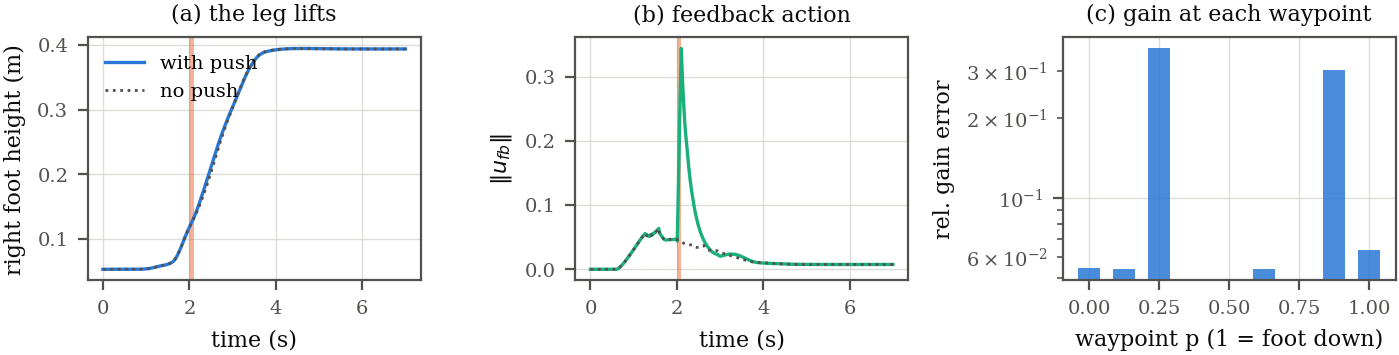
Three panels: right foot height with and without the push, norm of the feedback action, and the relative gain error at each waypoint
Fig. 9(a) the foot height with and without the push, which the controller absorbs. The tilt deviates by at most $2.6^\circ$ from its final value. (b) the feedback action is small during the lift and peaks when the push lands. (c) the relative gain error at the waypoints where the finite-difference Riccati solver returns a gain: $5.5\times10^{-2}$ at the one-leg end, $6.4\times10^{-2}$ at touch-down, and $0.3$ at two waypoints near the transition. At three other waypoints the reference solver fails and is left out, and at one the identified model itself is off by $0.47$ because the foot is just touching. Reading all nine gains out takes $23\,$s in total. The family needs one dataset per waypoint, so this is gain scheduling over nine set-points. It is not a single dataset serving every pose.

Unitree G1

The same pipeline runs on the Unitree G1, a 29-joint humanoid driven by joint torques, standing on both feet. The state has 70 dimensions and there are 29 torque inputs. Two details matter. The standing pose from inverse dynamics is not a rest point and the starting guess is far enough off that a plain Newton step diverges, so the set-point is refined with a trust region and a line search. And the model's joint dry friction has to go: a friction-loss constraint locks a joint at rest, so no small perturbation moves it and the linearisation sees no input at all. The offline data are short random-torque episodes around the set-point.
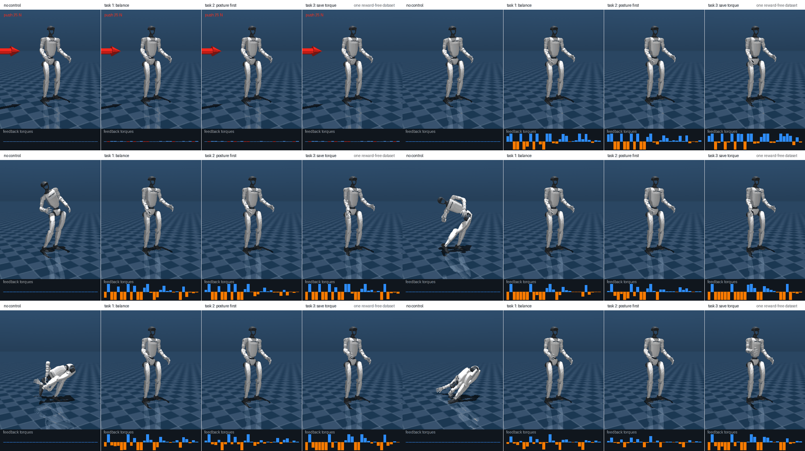
Unitree G1, n = 70, m = 29 500 Hz 40000 reward-free samples about 2 s / task
Four Unitree G1 robots standing after a 25 N sideways push; the uncontrolled one falls and the three with zero-shot gains hold
DemoA 25 N lateral push on the pelvis for 0.1 s, drawn as the arrow, played at half speed, with the feedback torque of each of the 29 motors below. Without control the robot falls. The three gains hold, and the torque dies away within a few seconds. 25 N is the largest push that all three absorb. The save-torque gain, which penalises torque three times as much, gives up first, at 50 N.
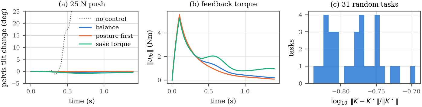
Three panels: pelvis tilt change after the push for the three tasks and the uncontrolled fall, the norm of the feedback torque, and a histogram of the relative gain error over random tasks
Fig. 10(a) the pelvis tilt after the push. (b) the norm of the feedback torque. All three gains settle, with the torque down to about $0.01\,$Nm after $5\,$s. (c) the relative gain error over $31$ random tasks that both solvers handle, with a median of $0.17$ and a worst case of $0.20$. For the three named tasks it is $0.23$, $0.20$ and $0.26$, much larger than in the smaller demos, although the identified model is within $6.5\times10^{-3}$ of the finite-difference one. The behaviour is what counts here: the balance gain recovers from pushes up to $75\,$N, exactly what the finite-difference Riccati gain does, posture first reaches $100\,$N and save torque $25\,$N. Policy iteration stops after $6$ to $9$ steps, at a step size of $10^{-6}$. Asking for $10^{-10}$ as in the smaller demos never terminates, because the root's translation and yaw sit at an eigenvalue of $1$ to within $10^{-5}$, so the Lyapunov solves are ill conditioned and the step stalls near $10^{-8}$. The closed loop on the finite-difference model has a spectral radius of $1.00007$ for the zero-shot gain, against $0.99993$ to $1.00000$ for the Riccati gain, so it is only marginal. In the simulator the deviations nevertheless shrink over $20\,$s, and the root's position and yaw offsets fall below $2\times10^{-3}$. A gain takes about $2\,$s to read out. Standing on one leg is the next case. Moving from two feet to one is not shown: a chain of rest points that shifts the weight over one foot stopped being a set of rest points after about $7\,$cm.

Unitree G1 on One Leg

My first attempt to find a single-leg rest point failed for a reason in the search, not in the robot. A Newton search that starts from the two-leg stance has to lift the right foot, and at lift-off the contact switches off, so the one-step velocity that the search tries to drive to zero is not smooth there. It stalled at a residual of about $10^{-1}$ whatever the target. The set-point is now built in three steps. First a smooth kinematic problem places the centre of mass over the left foot, with that foot fixed and flat and the right leg lifted. Then inverse dynamics gives the standing height and the torques. Then Newton steps on pose and torque remove what is left, from $2\times10^{-3}$ down to $8\times10^{-8}$. The result has the right foot $34\,$cm above the left, the centre of mass $3.8\,$cm from the left foot's centre and the pelvis tilted $16^\circ$.

The offline data need smaller excitation than on two feet. With the two-leg amplitudes the identified model is off by $1.7\times10^{-2}$, which is enough for the save-torque gain to destabilise the real system: it falls after a $3\,$N push and the closed-loop spectral radius is $1.0004$. At a tenth of the amplitude the model error is $2.0\times10^{-3}$ and all three gains hold. A gain that spends little torque has less margin to absorb model error, and a loop this close to the edge leaves very little.
G1 on the left leg, n = 70, m = 29 40000 reward-free samples about 2 s / task
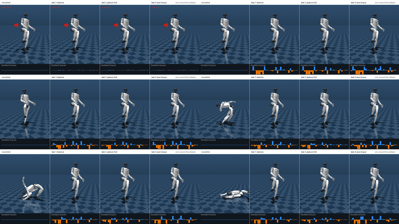
Four Unitree G1 robots standing on the left leg with the right leg raised, after a 10 N sideways push; the uncontrolled one falls and the three with zero-shot gains hold
DemoA 10 N lateral push on the pelvis for 0.1 s, drawn as the arrow, played at half speed, with the feedback torque of each motor below. Without control the robot falls, and the three zero-shot gains hold the pose on one foot.
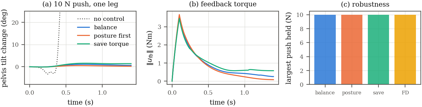
Three panels: pelvis tilt change after the push for the three tasks and the uncontrolled fall, the norm of the feedback torque, and the largest push each gain holds
Fig. 11(a) the pelvis tilt after the push. (b) the feedback torque. (c) the largest push each gain holds, on a grid of $5$, $10$, $20\,$N and up: all three gains and the finite-difference Riccati gain hold $10\,$N and none holds $20\,$N. Without a push the balance gain stays on the set-point for $10\,$s. The gains are within $0.09$ and $0.12$ of the Riccati gain for balance and save torque. For posture first the Riccati solver fails, so there is no reference. For the balance task and a $10\,$N push the zero-shot gain and the Riccati gain behave alike: the tilt peaks at $1.1^\circ$ against $1.0^\circ$, is at $0.29^\circ$ against $0.16^\circ$ after $2\,$s, and is back within $0.01^\circ$ by $5\,$s. A single narrow foot gives much less margin than two feet.

Unitree Go1 Quadruped

The last case is a quadruped, the Unitree Go1, one of the robots of the legged_control stack, standing on four feet. Here the gain acts at the torque level: the 12 joint motors are plain torque sources, with the reflected rotor inertia as joint armature and contacts only between the feet or body and the floor. The controllers of legged_control themselves, the OCS2 NMPC and the whole-body controller, are not used. The state has 36 dimensions. Four feet on the floor make the stance statically stable, so the set-point comes from inverse dynamics and a few Newton steps, and the finite-difference model is easy to match. The model error is $3.2\times10^{-3}$ with $40000$ samples, and a gain takes about $0.1\,$s to read out.
Unitree Go1, n = 36, m = 12 500 Hz 40000 reward-free samples about 0.1 s / task
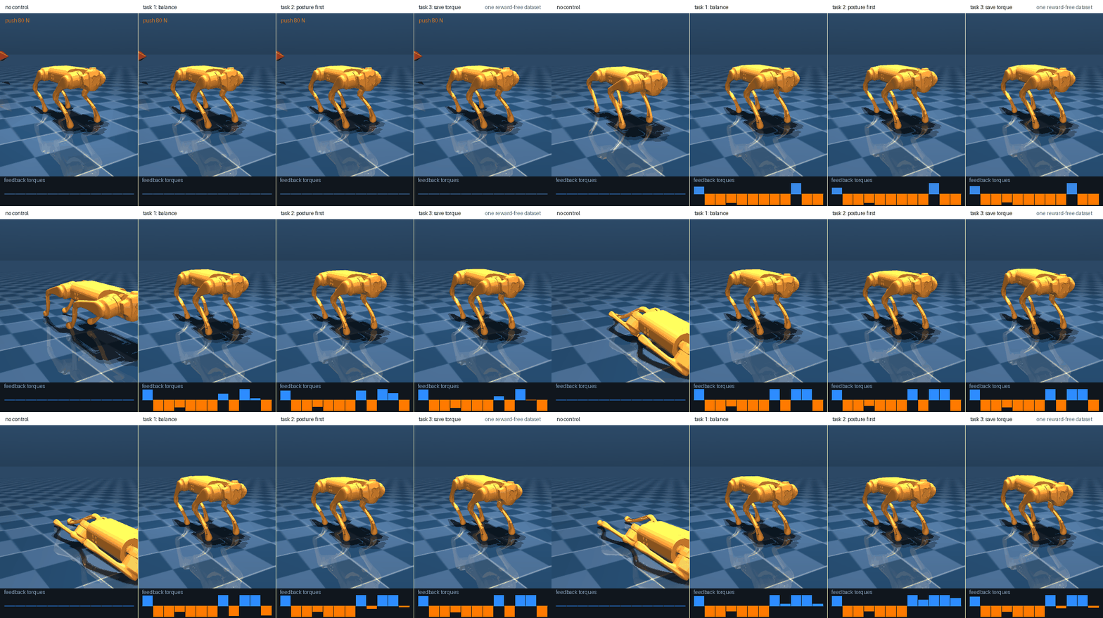
Four Unitree Go1 quadrupeds after an 80 N forward push on the trunk; the uncontrolled one collapses and the three with zero-shot gains stay standing
DemoAn 80 N forward push on the trunk for 0.1 s, drawn as the arrow, played at half speed, with the feedback torque of each of the 12 motors below. Without control the robot folds its legs and lies on the floor. The three gains, read out of the same reward-free representation, absorb the push and stay standing.
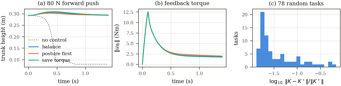
Three panels: trunk height after the push for the three tasks and the uncontrolled collapse, the norm of the feedback torque, and a histogram of the relative gain error over random tasks
Fig. 12(a) the trunk height after the push. The trunk tilt would not show the collapse, because the uncontrolled robot ends up flat and level. (b) the feedback torque. (c) the relative gain error over $78$ random tasks that both solvers handle, with a median of $2.3\times10^{-2}$ and a heavy tail, up to $0.69$ for the worst. For the three named tasks it is $2.7$, $3.6$ and $2.9\times10^{-2}$, and the gain is read out in $6$ to $8$ policy-iteration steps. Pushes of $0.1\,$s that each gain absorbs, forward and sideways: the balance gain $80$ and $60\,$N, exactly what the finite-difference Riccati gain does, posture first $150$ and $80\,$N, and save torque $80$ and $20\,$N. The thriftiest gain gives up first, as on the G1.

Go1 Walking

Standing is a fixed point, and walking is not. A trot is a limit cycle whose contacts switch on and off, so one linear model cannot describe it. The recipe here is periodic tracking of an orbit, and it is not a controller that invents the gait. The orbit comes from the simulator: a joint-PD controller follows foot trajectories generated by inverse kinematics (period $0.4\,$s, $0.29\,$m/s), and after a few seconds the closed loop settles on a periodic orbit. One period of states and applied torques, $200$ phases, is the reference.

For every phase the offline step collects its own short reward-free batch, $400$ one-step transitions with random deviations from the reference and random torques added to it, and keeps a fixed-size representation of that phase. A task $(Q,R)$ is then solved by the periodic backward Riccati recursion run on the $200$ representations alone, which gives one gain per phase, and the controller applies the recorded torque plus the gain times the deviation from the reference. The root's forward and sideways position is left out of the state, because the dynamics do not depend on it and the reference is for a moving robot. The finite-difference linearisation of each phase scores the result and is never used.

One change to the model was needed. With the stock contact parameters the one-step map has a jump at every touch-down, so a perturbation of $10^{-5}$ rad can change one step by a thousand times that, and no linear model fits. A softer impedance ramp removes the jump and leaves the gait as it was, $0.29$ against $0.30\,$m/s.
Go1 trot, n = 34, m = 12 200 phases x 400 samples 0.2 s / task
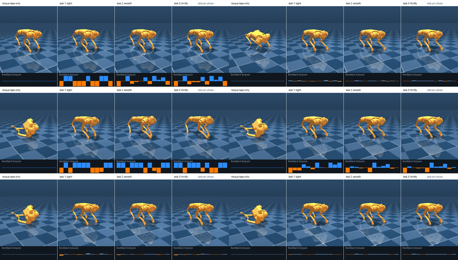
Four Go1 quadrupeds trotting after a 60 N sideways push; the one that only replays the torque tape falls and the three with zero-shot periodic LQR gains keep walking
DemoA 60 N sideways push on the trunk while trotting, drawn as the arrow, played at half speed. The first panel replays the recorded torques with no feedback and falls after $0.8\,$s. The other three add a gain read out of the per-phase representations, for three different costs, and keep walking.
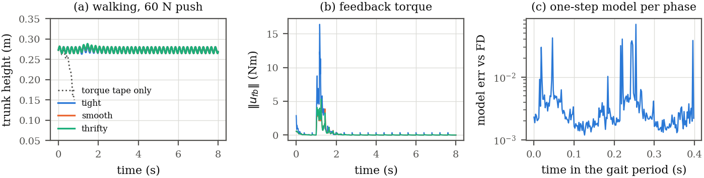
Three panels: trunk height while walking after the push for the torque tape alone and for the three gains, the norm of the feedback torque, and the one-step model error against finite differences at every phase of the gait
Fig. 13(a) the trunk height over $8\,$s of walking, with the push at $1\,$s. (b) the feedback torque, which dies away after the push. (c) the one-step model of each phase against the finite-difference one: median $2.3\times10^{-3}$, $95\%$ of phases below $9\times10^{-3}$ and the worst $6.9\times10^{-2}$, at the touch-down steps. Without feedback the period map has a spectral radius of $19.9$. The gains are within $1.5$ to $1.8\times10^{-2}$ of the finite-difference ones in median, and $1.4\times10^{-2}$ over $30$ random diagonal tasks, with a worst case of $2.1\times10^{-2}$. Each task takes $0.2\,$s. Pushes of $0.1\,$s at $1\,$s that the walk survives for $8\,$s, sideways and forward: the tight gain $150$ and $200\,$N, the smooth one $60$ and $200\,$N, the thrifty one $60$ and $100\,$N. The finite-difference gains give $150$ and $200$, $100$ and $60$, and $60$ and $100\,$N, and so the zero-shot gains match them for two tasks and differ in opposite directions for the third. The PD gait alone holds $60\,$N sideways and $200\,$N forward, so the tight gain is stronger sideways. The gait and its speed are fixed by the foot trajectories. The gain keeps the robot on the orbit, and it does not choose where to walk.

Go1 on a Circle

Walking along a path needs a reference that follows it. The simplest path that is still periodic is a circle: a steady turn is a limit cycle, once the state is seen from the circle. The trot tape gets longer strokes on the outside legs, the PD loop settles on an orbit with a constant yaw rate of $0.39\,$rad/s at $0.29\,$m/s, a circle of radius $0.74\,$m that takes $16\,$s to walk, and after one gait period of $0.4\,$s the whole state is the start state rotated about the centre of the circle. Everything else is as in the straight walk, with two changes that the turn needs. The root's position now stays in the state and gets a weight in the cost, since it is what brings the robot back to the circle after a push. And the measured state is rotated back about the centre by the angle that the reference has turned, so that the error is the one of the first period, for which the models were learned.
Go1 trot on a circle, n = 36, m = 12 200 phases x 400 samples 0.7 s / task
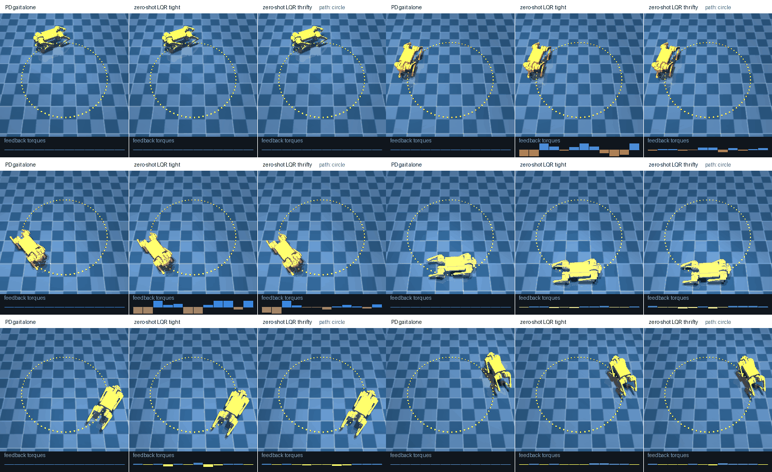
Top view of three Go1 quadrupeds trotting around a dotted circle after a 60 N sideways push at 3 s; the PD gait alone ends up on a displaced circle and the two with zero-shot gains return to the dotted circle
DemoThree robots trot around the dotted circle and take a 60 N sideways push on the trunk at 3 s. The PD gait alone, on the left, goes on around a displaced circle. The two with zero-shot gains, for the tight and the thrifty cost, walk back onto the dotted one.
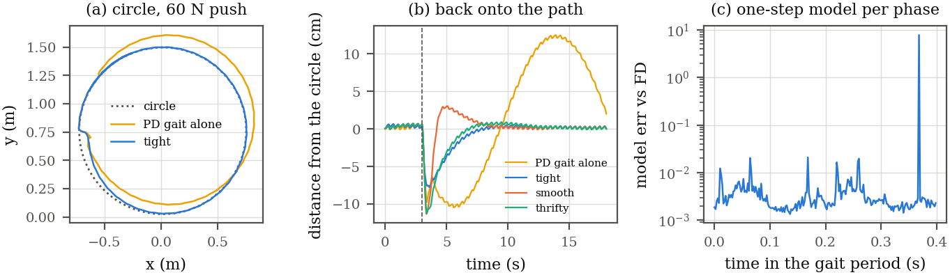
Three panels: the path of the PD gait alone and of the tight gain after the push against the circle, the distance from the circle over time for the PD gait and the three gains, and the one-step model error against finite differences at every phase
Fig. 14(a) the path after a $60\,$N push. (b) the distance from the circle. The PD gait ends up on a displaced circle and never comes back, so its distance swings between $-10$ and $+12\,$cm over each lap. The three gains are pushed off by $7.7$ (tight), $11.3$ (smooth) and $11.2\,$cm (thrifty), and each is back within $3\,$cm and stays there $2.0$ to $2.3\,$s after the push. The smooth one overshoots to the other side by $3.1\,$cm on the way. (c) the one-step model of each phase against the finite-difference one: median $2.6\times10^{-3}$, $95\%$ of phases below $8\times10^{-3}$, and one phase, the touch-down at $0.37\,$s, at $7.8$. The gains are within $2.3$, $4.3$ and $4.0\times10^{-2}$ of the finite-difference ones in median, and $5.3\times10^{-2}$ over $30$ random tasks with a worst case of $7.5\times10^{-2}$, a little worse than on the straight walk. Each task takes $0.7\,$s. Replaying the torques without feedback falls after $0.6\,$s. Pushes of $0.1\,$s at $3\,$s that the robot survives and returns from, sideways and forward: tight $100$ and $150\,$N, smooth $60$ and $60\,$N, thrifty $60$ and $60\,$N. The finite-difference gains give $100$ and $150$, $60$ and $60$, and $100$ and $60\,$N. The PD gait alone stays up to $60$ and $150\,$N but returns to the circle after none of them, since nothing in it measures where the circle is.

Franka Panda: Carrying a Block

The manipulator is a Franka Panda with seven torque-controlled joints, standing on a workbench with two stands under the corners of the path, so the state has 14 dimensions. A fully actuated arm has a rest point at every pose, holding it takes the gravity torque, and that is what inverse dynamics returns. The costs are in task space: a weight on the tool tip's position and orientation through the Jacobian, plus a weight on the joints. Holding the ready pose, the model identified from $15000$ samples is within $2.8\times10^{-4}$ of the finite-difference one, and the gains for three tasks are within $5.0\times10^{-3}$, $1.2\times10^{-2}$ and $8.7\times10^{-3}$ of the Riccati ones, each after $9$ to $12$ policy-iteration steps in about $0.1\,$s. Over $200$ random tasks the median is $2.0\times10^{-2}$ and the worst case $8.1\times10^{-2}$.

The harder case moves. A $1.5\,$kg block is held between the fingers, rigidly fixed to the hand, and the tool tip carries it along a loop that lifts it, moves it over $0.5\,$m, lowers it and comes back, $8.4\,$s in all, with a stop at each corner. Every pose of the path is a rest point only while the arm is still, so the reference is a trajectory: the joint angles from inverse kinematics and the torque tape from inverse dynamics. Along it the offline step keeps a representation every $0.05\,$s, $168$ of them with $300$ one-step transitions each, and a task is solved by the periodic Riccati recursion over the loop on those representations alone, as for the quadruped's gait. The torque tape alone would hold the tip to $0.05\,$cm for the first second. The mass of the block is not given to the algorithm. It is in the data.
Franka Panda, n = 14, m = 7 168 knots x 300 samples 0.5 s / task
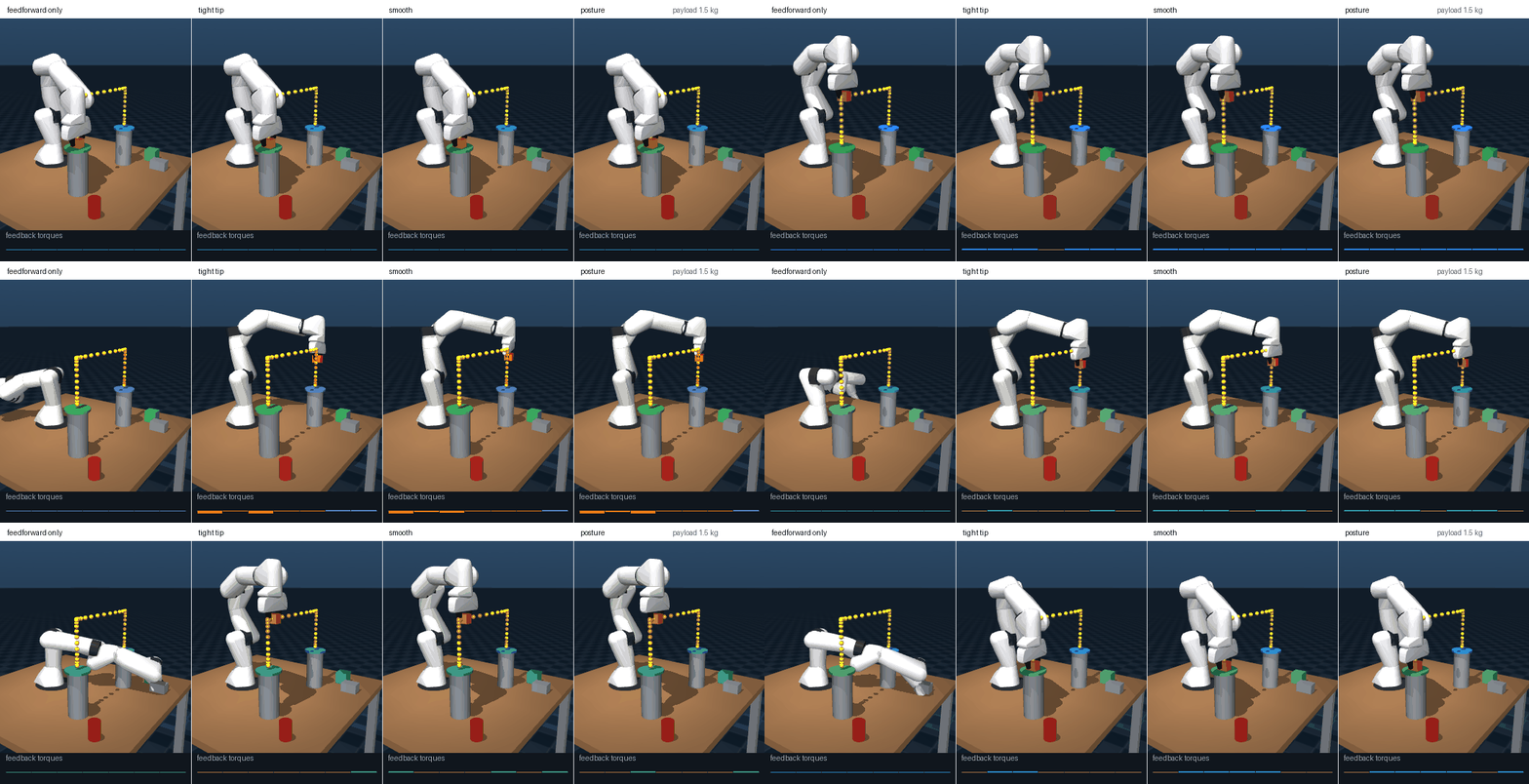
Four Franka Panda arms carrying a block along a dotted path after a 40 N push on the hand at 3 s; the arm with the torque tape alone collapses and the three with zero-shot gains return to the path
DemoThe arm carries the block along the dotted loop and takes a 40 N sideways push on the hand at 3 s. With the torque tape alone, on the left, it collapses. The three arms with gains read out of the per-knot representations, for three different costs, come back onto the path. The strip under each arm shows the feedback torque of each of the seven joints.
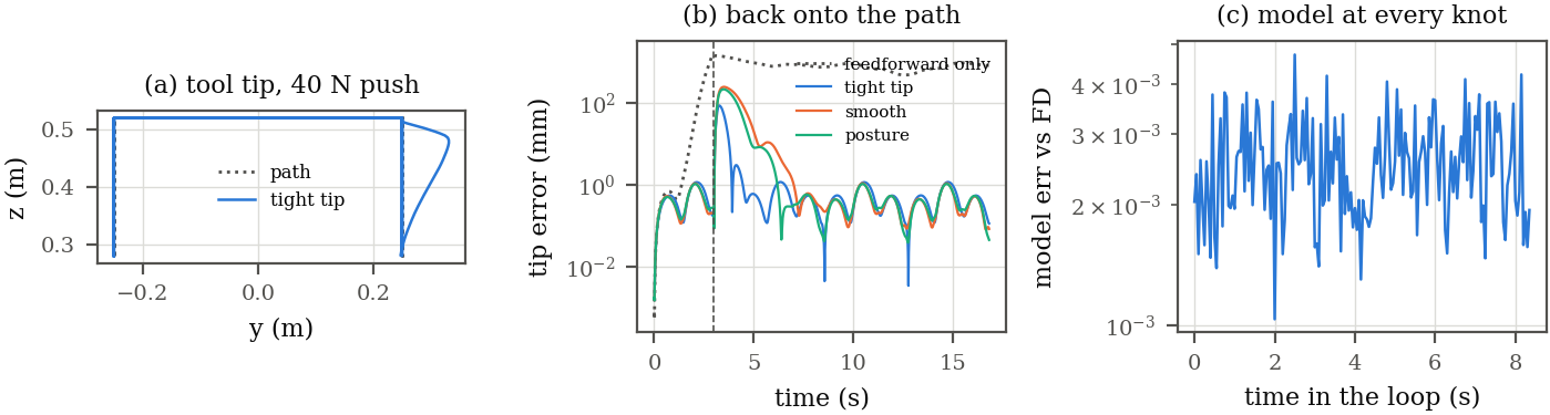
Three panels: the path of the tool tip of the tight gain after the push against the loop, the tip error over time for the torque tape alone and the three gains, and the one-step model error against finite differences at every knot
Fig. 15(a) the tool tip of the tight gain, which swings out at the push and comes back. (b) the tip error: without feedback it goes to $1.4\,$m, and with any of the gains it returns to the sub-millimetre error of the tracking itself, about $0.5\,$mm. (c) the one-step model at each knot against the finite-difference one, between $10^{-3}$ and $5\times10^{-3}$. The periodic gains are within $6.6$, $5.6$ and $4.8\times10^{-2}$ of the finite-difference ones in median and take $0.5\,$s each. The peak tip error after a push of $20$, $40$, $60$ and $80\,$N is $42$, $84$, $126$ and $167\,$mm for the tight gain, $126$, $238$, $334$ and $415\,$mm for the smooth one and $109$, $209$, $296$ and $373\,$mm for the posture one, and the finite-difference gains give the same to within $2\%$. The error grows in proportion to the push, and the cost sets how far the arm gives way. This is a transport of a block that is held, with no grasp and no contact. The reference torque comes from the simulator's inverse dynamics, as the set-points of the other demos do.

Machine-Precision Exactness, Constant Test-Time Cost, Predicted Sample Complexity

A single reward-free dataset solves 200 random LQR tasks to machine precision. SF-GPI closes most of the optimality gap without solving any equation at test time. The predicted $1/N$ sample-complexity rate holds across three excitation levels.
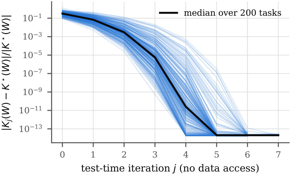
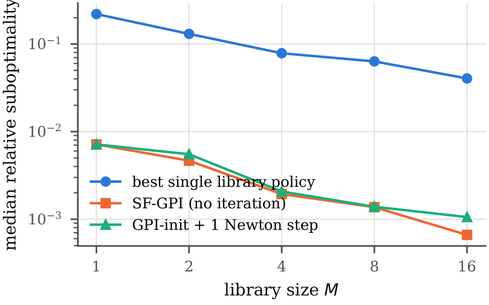
Rosenbrock batch reactor n = 4, m = 2 open-loop unstable 200 random tasks N up to 5000

Table 1. Per-task test-time cost against per-task off-policy Q-learning on the same reward-free data (mean over 20 tasks)

NOffline (ms)Zero-shot (ms)Off-policy QL (ms)
2000.050.3714.5
10000.080.3973.3
50000.140.39358.5

The zero-shot test-time cost stays flat at $\sim\!0.4\,$ms as $N$ grows $25\times$. Per-task off-policy Q-learning on the same data grows linearly with $N$. Both methods return the same gains, to within $2.2\times10^{-13}$–$1.4\times10^{-12}$.

Table 2. Task inference from noisy reward labels instead of $(Q,R)$ (50 tasks, $N=1000$)

Label noiseMedian weight errorMedian subopt.Worst subopt.
0%$1.7\times10^{-14}$$\approx 0$$3.3\times10^{-14}$
1%0.020$4.6\times10^{-5}$$3.0\times10^{-3}$
10%0.204$5.5\times10^{-3}$0.168
100%2.120.1911.76

Noise-free labels identify the task weights exactly. Even $1\%$ label noise leaves the median suboptimality at $4.6\times10^{-5}$, because the LQR solution tolerates moderate weight errors. Specifying a task by reward labels is therefore practical.

Citation

@misc{dao2026zeroshotlqr,
  title={Zero-Shot Linear Quadratic Regulation from Reward-Free Data: Structured Successor Features with Stability and Finite-Sample Guarantees},
  author={Dao, Huy and Thai, Khanh and Le, Bao},
  year={2026}
}